How to optimize life and work – or at least your coffee intake: numerical optimization in engineering
Everybody encounters dilemmas on a daily basis. Should you take the bus or the tram to work? Is it cheaper to drive a gasoline, diesel or even an electric car? How many cups of coffee do I need to write the best code?
Whenever you come across a problem, you are presented with a choice. Most choices are made subconsciously, based on experience and knowledge. Others, such as buying a new car, usually involve some research as the financial aspects may have a significant influence on your daily life.
Typically, we don’t make the optimal choice as real-life problems are often complex and influenced by many factors. Finding an optimal diet, for example, not only requires profound knowledge of nutritional value of foods and human physiology, but you would also need to know what kinds of food someone likes to eat.
One of the things I love most about engineering is that we actually have the tools available to make optimal decisions and take the fuzziness of choices out of the equation. Compromises are captured in the problem itself and no better solution than that of the optimization problem exists. So… how is this done? In a nutshell, we need a cost function, models and a solver.
The cost function
Every optimization involves a cost function. Let’s start with an example and express my productivity, expressed as € earned per hour for my employer with respect to the cups of coffee I consume during the day:
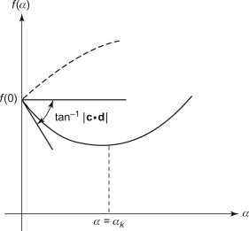
In the figure above you can see that I need at least a few cups of coffee before I become productive, but that drinking too much coffee just means that I’m hanging around the coffee machine all day.
For this problem, the cost function is directly related to the underlying model of my productivity versus my coffee intake, which is basically a second order polynomial here. A few evaluations of this function for different cups of coffee by an appropriate solver quickly reveals that the optimum is found around 4-5 cups.
However, the cost function becomes more complex and interesting when we are looking at several metrics simultaneously. Suppose we consider buying a new car again. In this case, we don’t only want to reduce our fuel usage, but also our CO2 emissions. Now the cost function to be minimized can be formulated as a function of both metrics: cost = aconsumption + bCO2. The exact values of consumption and CO2 emissions are based on models taking into account the weight of the car, its engine power or fuel type. a and b can be tuned to put more weight on consumption or emissions.
Sometimes the problem itself is more complex than the cost function. A well known example is that of the traveling salesman. The salesman wants to know the fastest route between multiple points in a city with bridges, one-way traffic and other obstacles. While the cost function is just expressed as the time or distance spent traveling, the problem requires a model that find this value for any possible route.
The models
So how do we get to know the values needed for the cost function? For this we need models. Models can be as simple as a spreadsheet listing a number of cars with consumption and emissions figures or as complex as a complete computer simulation of a vehicle based on a set of parameters, such as weight, air drag coefficient, (this is a very, very long list…). The complex model can include finite element modelling techniques such as computational fluid dynamics for the air drag or structural analysis for the suspension dynamics.
An example of a rather simple model is the BMI model. Based on your body weight, length and your age, the BMI can be calculated. The metric is the BMI itself and you’d want to optimize this to be as close to a healthy value as possible. Since we can’t really influence our length or age, the one parameter that we can optimize in this regard is our weight, but nobody said optimization is easy…
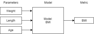
All we want from a model, is for it to take some given parameters and to receive in return the metrics which are used in the cost function. For the traveling salesman problem it requires us to provide any combination of parameters that completes a route. For the BMI calculation it’s just the three parameters.
The solver
Now that we have our cost function and our model, we can use an algorithm to find the optimum for us. This algorithm is typically called a solver. The most straightforward solver is perhaps simulating all possible combinations of parameters and picking the combination that provides the best cost. For the spreadsheet with cars, for example, this is quite feasible. For the complex car model featuring the computational fluid dynamics and structural analysis or the traveling salesman however, it isn’t. When the model becomes more complex, it takes longer to simulate a single combination of parameters, and that is where the difference can be made with a solver.
The first type of solvers we’ll discuss here are so called convex solvers for convex functions. Wikipedia gives a much better explanation than I could, but here it suffices to say that a convex function is a function which keeps improving the cost in one direction with respect to the parameter until it reaches the optimum. The cups of coffee example is a convex function: when you start at a point which is not the optimum, there’s only one way to the optimum. Convex solvers are typically very fast, but unfortunately, not all our problems are convex.
Most problems are actually non-convex and require a global solver. To understand a non-convex model, suppose you start in the Alps in Austria and want to reach the highest peak of the Alps. You can change your coordinates (parameters) by walking, the evaluation of the model and cost function returns the height you’re currently at. When you approach this as a convex problem, you’d just start walking up the closest hill until you are at its peak. Just looking down from this peak you see that there is no way for going up any further, but when you look around you can see the Mont Blanc in the distance, surely being higher than the hill you just climbed. Global solvers have various ways to occasionally descend until you start at the foot of Mont Blanc and climb until you are at the actual highest peak in your solution landscape.
What I find fascinating about global solvers is that some are based on natural processes such as annealing of metals (simulated annealing), evolution (genetic algorithm) or even the movements of ant colonies (ant colony optimization) and provide great results.
Optimization in your life
Whether your problem is easy or complex, it can be optimized in one way or another. With today’s computational capacity and production technologies, more and more designs can be created and realized. Below is an example of a chair developed using topology optimization.

Hemmerling, M., & Nether, U. (2014). Generico-A case study on performance-based design.
Perhaps without even knowing it, you’re using many optimized technologies. Every microchip or PCB has gone through an extended optimization phase to fit as many transistors and electrical components on a small footprint. Every app on you phone is optimized for resource usage (battery and processor). Each time you use your satnav in a car, the route is optimized to keep you out of traffic jams and home as fast as possible (like the traveling salesman). Whether it’s for the best or not that your data is used in optimization algorithms by the large service provides remains a challenging question, but that it’s happening is no secret.
The only question that remains is: “what can you do to further optimize the world and how would you define its cost function?”
About the authors