Servo-Drive Mechanism Design: A Simulation-Led Workflow from Motion Requirement to Detailed Design

A methodology for sizing and validating high-speed, cyclic servo-driven transfer mechanisms using multibody dynamics, motor sizing, drivetrain studies, and bearing / FEA verification.

Abstract

Mechanical transfer mechanisms driven by servomotors, indexing slides, transfer fingers, linkages, and similar cyclic devices are common in high-throughput production machinery. Sizing the motor, drivetrain, and structural components correctly the first time avoids costly rework late in a project. This article describes a design workflow, developed and applied in an industrial R&D setting, that moves systematically from a preliminary concept through multibody dynamic simulation, motor sizing, drivetrain trade-off (belt-and-pulley versus direct coupling), bearing selection, and finite-element verification, closing with an iterative update loop that keeps the simulation and the physical design synchronized.

Introduction

High-speed cyclic mechanisms (Fig:1) place unusual demands on their drive components. Main components are servo-motor, crank-arm, connecting rod and slider. The only known parameter is the target-slider-profile (It is the slider position vs time graph). We have the CAD and material information about the slider but all other parameters are unknown.

The motor must deliver a torque profile that changes rapidly within a single cycle, bearings see fluctuating and sometimes reversing loads at a high duty cycle, and the structural frame must avoid resonance with the actuation frequency. Getting the sizing right requires more than a static torque calculation: the inertia of the moving assembly, the kinematics of the mechanism, and the effects of friction all vary continuously through the stroke and must be captured together, not estimated independently.

The workflow below was developed to make that sizing process repeatable and auditable. It separates the problem into a chain of well-defined stages, each with a clear input, output, and acceptance check, and it builds in an explicit return path so that new information from analysis or detailed design can flow back into earlier assumptions rather than being handled as an ad hoc exception.

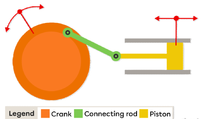
Fig 1: Cyclic servo-driven transfer mechanism

Overall Workflow

The diagram below summarizes the process end to end. It begins with a preliminary mechanical concept and a multibody dynamic model, proceeds through motor and drivetrain selection, and only then opens into detailed design (CAD, FEA, fatigue, and fastening). A design-change review step is built in so that findings from detailed design or FEA can trigger either a local update or, if the change is significant, a full return to the multibody model.

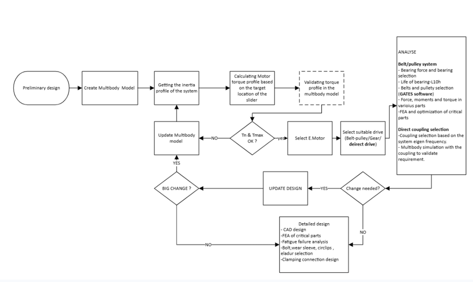
Figure 1 — Generalized design workflow for a servo-driven mechanism, from preliminary concept to detailed design.

Preliminary Design and Multibody Dynamic Modelling

The process starts from a preliminary mechanical concept: a proposed linkage or slide geometry, an assumed material set, and the resulting mass and inertia distribution taken from CAD. This concept is translated into a multibody dynamic model in Simscape(MATLAB) that captures the kinematics of the mechanism. Multibody is very detailed with the dimension of parts, links and joints. For the unknown parts, values of inertia and mass were taken into consideration along with the safety margin. 

Deriving the inertia profile

The multibody model is exercised through a full motion cycle to extract the reflected inertia of the system as seen at the motor shaft, as a function of motor angle. Because most transfer and indexing mechanisms are not simple constant-ratio drives, this reflected inertia is rarely constant through the stroke. It typically varies with the instantaneous mechanism geometry, so a single ‘equivalent inertia’ number is not sufficient for sizing. The varying inertia profile of the whole system was easily calculated from the multibody model as the function of servo angle.

Motion law and required torque

A target motion law (position, velocity, and acceleration versus time) is defined for the output member, based on the required cycle rate and any process constraints on velocity or acceleration at pick-up and drop-off points. Combining this motion law with the inertia profile from the multibody model gives the required motor torque as a function of time. Since the reference-motion-target and inertia is known, various mathematical methods are used to get the torque profile. Few of the methods are below:
1. Jerk-limited S-curve trajectory
2. Minimum-Jerk Optimization
3. Minimum-Torque-Change Optimization
4. Optimal Control / Model Predictive Control (MPC)

After using one of the above methods was implemented in MATLAB codes which calculated motor torque, peak and nominal (duty-averaged or RMS) torque and speed requirements..

Model validation

Before the torque profile is used for motor sizing, the multibody model itself is validated. One effective check is a round-trip comparison: the torque profile calculated from the motion law is fed back into the multibody model as an input. Slider profile is the output of the model and is compared with the reference-slider-profile. Only when this comparison/ validation closes within an acceptable tolerance, the torque profile gets carried forward into motor selection. This step is cheap relative to hardware iteration and catches modelling mistakes — sign errors, missing inertia terms, incorrect joint definitions — before they propagate into a motor or drivetrain that is either oversized (cost) or undersized (cannot meet the cycle rate).

Motor Selection

The peak and nominal torque and speed requirements from the validated multibody model are used to screen candidate servomotors. Because raw simulation output from a dynamic model is often noisy (numerical differentiation of position to get acceleration is a common source), the torque signal is filtered or averaged before nominal-torque values are extracted, while peak values are read directly from the unfiltered signal since transient peaks are physically real and should not be smoothed away.

Candidate motors are compared on a torque-speed plot against their nominal-torque curve (which is speed-dependent and falls off at higher speed, not a flat rated value) and their peak-torque limit. A simple pair of acceptance criteria keeps some design margin in hand:

Criterion	Typical acceptance margin
Calculated nominal (RMS) torque	≤ ~y% of motor rated torque
Calculated peak torque	≤ ~z% of motor peak torque
Nominal torque vs. speed	Checked against the motor’s speed-dependent nominal-torque curve, not a single rated point

These margins are deliberately conservative: they leave headroom for friction effects not yet included at this stage of the analysis, for future speed-up of the cycle rate, and for the normal uncertainty in an early-stage inertia and mass estimate.

Refining the Load Model: Friction

The multibody model up to this point is frictionless. Real sliding mechanisms are not: preloaded contact surfaces (for example a leaf-spring preload used to remove backlash) introduce a friction force proportional to the local normal force, and this friction acts in more than one direction depending on the mechanism architecture. The friction model was integrated in the multibody model. The results showed negligible impact on the motor torque and its selection.

A secondary observation from this stage: because the multibody model idealizes the slide as perfectly rigid and uniformly loaded, some additional friction from non-uniform loading (e.g., slight bending of a long linear guide) may exist in the physical system but is not captured by simulation. Where this matters, it is best resolved by correlating the model against instrumented test data rather than by further refining the idealized model. Therefore, it is always better to have a lower acceptance margin (section 4) on the motor torque selection.

Drivetrain Selection: Belt-and-Pulley vs. Direct Coupling

With the torque and speed requirement established, a drivetrain architecture is chosen. Two options are commonly compared for this class of mechanism:

• Belt-and-pulley (or gear) reduction
• Direct coupling

Belt-pulley option: A belt-and-pulley drive was evaluated first, using belt-sizing software to check the available belt types and pulley combinations against the system’s torque requirement. This showed a problem: because the torque requirement was fairly high, the belt and pulley components needed to handle it were themselves large and heavy. That extra rotating mass added meaningfully to the system’s inertia on top of what the mechanism already required. As a result, the motor had to be upgraded to a bigger, considerably more expensive unit, just to compensate for the inertia the drivetrain itself had added. Combined with the larger physical size of the belt-pulley hardware, this made the belt drive a poor fit for a prototype where both cost and size mattered.

Direct coupling option: Direct coupling was analysed as the alternative. Several coupling types were compared, with the choice coming down mainly to four criteria: rotational-inertia, nominal torque capacity, operating speed, and the torsional stiffness of the coupling. Since a direct-drive system has no belt or gear stage to absorb torsional vibration, the coupling itself becomes the critical link. The torsional eigenfrequency of the coupled system was checked in detail using the multibody model, to confirm it stayed well clear of the mechanism’s operating frequency. All these four criteria met our requirement and direct coupling was selected.

The multibody model turned out to be useful beyond just sizing the motor. Because it already existed, checking a completely different drivetrain option — belt versus direct coupling — was quick. The same model could be reused with the coupling swapped in, so the eigenfrequency question was answered directly instead of starting a new analysis from scratch. This made the final decision faster and gave more confidence in the result.

Bearing Selection

Each support bearing in the load path is sized against the local reaction force computed from the multibody model (static and dynamic loading). For a typical mechanism with several bearing locations along its load path, the type of bearing needed differs by location. For example, some positions carry combined radial/axial load, while others (bushing-type supports) are chosen specifically because they can be continuously lubricated in service.

Load calculation methods

Bearing reaction forces can be worked out using more than one method, and some are more conservative than others — for example, a simple static free-body calculation versus a method that accounts for the equivalent dynamic load from a full cyclic force history and the equivalent rotational speed. As a general guide, a static calculation is usually adequate when speed and load are both low, while a dynamic calculation is important whenever the bearing load varies significantly during the cycle. Bearing manufacturers’ websites, such as SKF’s, provide detailed guidance on how to carry out these calculations.

Bearing life and type selection

Selected bearings are checked against the standard L10h basic rating life calculation using the equivalent dynamic load from the previous step and the operating speed profile. For mechanisms with significant angular acceleration as opposed to steady rotation, bearing type selection deserves particular attention. Rapid acceleration introduces failure modes that a simple static load rating does not capture:

Loading condition	Favourable bearing type	Key risk at high acceleration
Heavy combined radial/axial load, moderate acceleration	Tapered roller bearing	Roller skidding, preload sensitivity, cage stress during transients
High radial acceleration, low axial load	Cylindrical roller bearing	Poor axial capacity if load path changes
Very high acceleration / high speed	Angular-contact ball bearing (often paired)	Needs correct preload to avoid skidding
Extreme acceleration, high speed, thermal sensitivity	Hybrid ceramic angular-contact bearing	Higher cost; used selectively

As a general rule drawn from bearing-manufacturer guidance, adequate preload is important in high-acceleration angular-contact applications specifically to prevent roller/ball skidding during rapid transients. It is a failure mode that shows up as surface smearing rather than classical fatigue, and is not predicted by an L10h calculation alone.

Detailed Design and Structural Verification

Once the motor, drivetrain, and bearings are selected, the project moves into detailed design. This stage converts the sized components into a complete CAD assembly and adds the mechanical design work that a multibody or belt-sizing tool does not cover:

• Finite-element analysis of critical structural parts (chassis, base, slide) under the peak loads derived from the multibody model, including checks of assembly stiffness and any welded-joint sequencing needed to control distortion.
• Fatigue analysis of components subject to the full cyclic load history, not just the peak load  relevant for any part that sees millions of reversing load cycles over its service life.
• Selection of secondary machine elements: shaft seals, wear sleeves, retaining rings (circlips), and the fasteners in any clamped/bolted joint, each sized against the loads and tolerances established earlier in the process.
• Clamped-connection (bolted-joint) design, including the required clamp/tensile force in the bolts and the resulting bolt selection, following standard bolted-joint design theory.
• Where slender structural members are loaded in compression, a buckling check is added alongside the strength check.

Bearing fits are re-checked at this stage against the actual detailed-design tolerances (shaft and housing fit classes), since the effective internal clearance of a bearing after a tight fit can differ from its as-supplied clearance — a detail that is easy to lose track of between the bearing-selection stage and final drawings. Also, it is very important to note that the static, dynamic/fatigue loading data is all got from the multibody model.

The Iteration Loop

Detailed design and FEA often turn up things the earlier steps didn’t expect — a clash between parts, an unwanted vibration, or a load path that’s stiffer or more flexible than assumed. Instead of just patching these issues one by one, the process asks a clear question each time: is this a small local fix, or does it change something the earlier steps assumed?

• Small findings are handled in an “update design” step and stay within detailed design.
• Bigger findings are ones that change the load path, the weight or inertia of moving parts, or the drivetrain which go all the way back to “update the multibody model,” so the torque and speed numbers, and everything based on them, get recalculated properly instead of patched.

This matters because it’s exactly the kind of call that’s easy to get wrong under time pressure. A change that looks small, like swapping a bearing, can quietly shift the system’s inertia or stiffness enough to make the earlier motor sizing wrong. Building this decision point into the process, rather than leaving it to whoever notices the issue, makes the risk visible and gives the project a clear reason to either fix it locally or redo the earlier steps.

Discussion

A few parts of this process are useful beyond the specific mechanism it was built for:

• Check the model before using it. Testing the multibody model both ways — torque in, motion out, and motion in, torque out — before trusting it for motor sizing is a small extra step. It catches a lot of modelling mistakes early, while they’re still cheap to fix.
• Add complexity one step at a time. Adding friction, or any other secondary effect, one source at a time and checking its actual impact avoids two problems: missing something that matters, and overloading the model with detail that doesn’t change the answer but slows down every future run.
• Don’t lock in the drivetrain too early. Treating the choice between belt drive and direct drive as something that can be revisited — with a clear path back through the bearing and coupling checks — avoids getting stuck with an early choice that later turns out to be wrong.
• Make change-routing explicit. Deciding clearly whether a change stays local or forces a redo of earlier steps, as a set step rather than a judgement call made in the moment, carries over easily to other design projects with a similar simulate-select-check process.

None of this replaces engineering judgement. Choosing which bearing-load method to trust, deciding whether a friction effect is worth keeping, and deciding what counts as a “big” change all still need an experienced engineer. What this process does is make those judgement calls visible, repeatable, and easy to revisit as new information comes in.

Conclusion

Sizing a servo-driven cyclic mechanism correctly requires treating motor selection, drivetrain design, bearing selection, and structural verification as one coupled problem rather than a sequence of isolated calculations. A multibody dynamic model, validated before it is trusted, provides the common thread that ties these stages together and gives each downstream decision motor torque/speed rating, drivetrain architecture, bearing type and life, structural loading – a consistent and traceable basis. Just as importantly, building an explicit iteration loop into the process, with a clear rule for when a finding stays local versus when it must propagate back to the dynamic model, keeps the design internally consistent even as it inevitably changes over the course of a project.